Signal Compressing and Decomposing
This example is based on the work of Morlet and Grossman. The example deals with a signal of birthrates from 1944 to 1951. We will convert the signal into wavelet coefficients, compress the signal using hard thresholding, and then recompose the signal to compare it to the original (the new one will be slightly altered).
The birthrates from 1944 to
1951 can be organized as a signal of length 8 and turned into a vector.
> Birthratesignal:=[156.7,143.3,189.7,212,200.4,201.8,200.7,215.6]:
> f:= (i) -> Birthratesignal[i]:
> birthratesignal:=Vector(8,f);
Next, we will organize the birthrates into ordered
pairs with their corresponding years.
> for i from 1 to 8 do brp[i]:=birthratesignal[i]: od:
> Birthratepoints:= [[ n+1943,
brp[n]] $n=1..8];
![]()
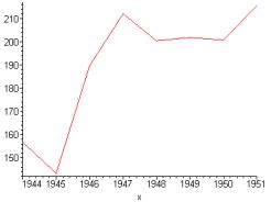
Notice the plot of these birthrates shown below.
> plot(Birthratepoints, x=1944..1951, style=line,symbol=circle);
Next, we can process the signal into wavelet
coefficients using the matrix of the Haar wavelet family, which we discussed
earlier.
> A3:=Transpose(Matrix([[1,1,1,1,1,1,1,1],[1,1,1,1,-1,-1,-1,-1],[1,1,-1,-1,0,0,0,0],[0,0,0,0,1,1,-1,-1],[1,-1,0,0,0,0,0,0],[0,0,1,-1,0,0,0,0], [0,0,0,0,1,-1,0,0], [0,0,0,0,0,0,1,-1]]));
> f:= (i) -> brp[i]:
> brp:=Vector(8,f);
> wc:= LinearSolve(A3, brp, method='QR');
Next, we will compress our signal (slightly change our wavelet coefficients) using hard thresholding. For this type of thresholding, we take the absolute value of our wavelet coefficients and if their absolute value is below a certain set number we turn the wavelet coefficient to zero. Let’s chose 8 for our number. Therefore, any wavelet coefficient whose absolute value was less than 8 will be turned to 0.
> for i from 1 to 8 do
> if abs(wc[i]) < 8 then wc[i]:=0: fi: od:
> wc;
Next, we can recompose our signal by taking these
altered wavelet coefficients and multiplying by our A3 matrix. This will give us a new signal that is only
slightly different from our original signal.
> brpnew:=Multiply(A3, wc);
Now, below we can compare the original signal to our
new signal.
> brp, brpnew;
Now, we can organize our new signal into ordered
pairs in order to graph it.
> Birthratepointsnew:= [seq([ n+1943, brpnew[n]], n =1..8)];
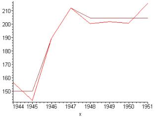
Finally, by looking at the graphs of our two
signals, we can see that Morlet and Grossman were right. Changing the wavelet coefficients slightly
only alters the recomposed signal a little bit (the original signal is red, and
the recomposed signal is brown).
> plot({Birthratepoints, Birthratepointsnew}, x=1944..1951, style=line,symbol=circle, color=[red, brown]);